The Idea
A few months ago I read a paper with the title “Deep Neural Networks Are More Accurate Than Humans at Detecting Sexual Orientation From Facial Images”, which caused a lot of controversy. While I don’t want to comment on the methodology and quality of the paper (that was already done, e.g. in an article by Jeremy Howard), I found it very interesting and inspiring. In a nutshell, the researchers collected face pictures from dating websites and built a machine learning model to classify people’s sexual orientation and reached quite an impressive accuracy with their approach.
This guest post summarizes the results as:
AI Can’t Tell if You’re Gay… But it Can Tell if You’re a Walking Stereotype.
And indeed, we often see people who look very stereotypical. I tried to think of more such scenarios and came to the conclusion that another environment, where this phenomenon can be found quite often, is a university campus. So often you walk around the campus and see students, who just look like a law student, a computer science nerd, a sportsman, etc. Sometimes I’m so curious that I almost want to ask them whether my assumption is correct.
After having read the above paper, I wondered if some machine learning model might be able to quantify these latent assumptions and find out a stereotypical-looking student’s profession or major.
Although I only have a little more than basic knowledge in machine learning, especially in image classification using deep neural nets, I took it as a personal challenge to build a classifier, that detects academics’ major based on an image of their face.
Disclaimer
Please don’t take this article too serious. I’m not a machine learning expert or a professional scientist. There might be some mistakes in my methodology or implementation. However, I’d love to hear your thoughts and feedback.
Approach
My first (and final) approach was to (1.) collect face pictures of students or other academics, (2.) label them with a small, limited set of classes, corresponding to their major, and eventually (3.) fit a convolutional neural net (CNN) as a classifier. I thought of fields of study, whose students might potentially look a bit stereotypical and came up with four classes:
- computer science (~ cs)
- economics (~ econ)
- (German) linguistics (~ german)
- mechanical engineering (~ mechanical)
Please note that this is not meant to be offending by any means! (I’m a computer science nerd myself 😉).
Getting the data
The very first prerequisite is training data - as usual, when doing machine learning. And since I aimed at training a convolutional neural net (CNN), there should be a lot of data, preferably.
While it would have been a funny approach to walk around my campus and ask students for their major and a picture of their face, I would probably not have ended up with a lot of data. Instead, I decided to crawl pictures from university websites. Almost every department at every university has a page called “Staff“, “People”, “Researchers” or the like on their websites. While these are not particularly lists of students, but of professors, research assistants and PhD candidates, I presumed that those pictures should still be sufficient as training data.
I wrote a bunch of crawler scripts using Python and Selenium WebDriver to crawl 57 different websites, including the websites of various departments of the following universities:
- Karlsruhe Institute of Technology
- TU Munich
- University of Munich
- University of Würzburg
- University of Siegen
- University of Bayreuth
- University of Feiburg
- University of Heidelberg
- University of Erlangen
- University of Bamberg
- University of Mannheim
After a bit of manual data cleaning (removing pictures without faces, rotating pictures, …), I ended up with a total of 1369 labeled images from four different classes. While this is not very much data for training a CNN, I decided to give it a try anyway.
Examples
Images
An excerpt from the folder containing all raw images after crawling: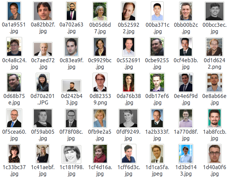
(If you are in one of these pictures and want to get removed, please contact me.)
Labels
An excerpt from index.csv containing labels and meta-data for every image:
1 | id,category,image_url,name |
Preprocessing the data
Before the images could be used as training data for a learning algorithm, a bit of preprocessing needed to be applied. Mainly, I did two major steps of preprocessing.
- Cropping images to faces - As you can see, pictures are taken from different angles, some of them contain a lot of background, some are not centered, etc. To get better training data, the pictures have to be cropped to only the face and nothing else.
- Scaling - All pictures come in different resolutions, but eventually need to be of exactly the same size in order to be used as input to a neural network.
To achieve both of these preprocessing steps I used a great, little, open-source, OpenCV-based Python tool called autocrop with the following command:
autocrop -i raw -o preprocessed -w 128 -H 128 > autocrop.log.
This detects the face in every picture in raw folder, crops the picture to that face, re-scales the resulting image to 128 x 128 pixels and saves it to preprocessed folder. Of course, there are some pictures in which the algorithm can not detect a face. Those are logged to stdout and persisted to autocrop.log.
In addition, I wrote a script that parses autocrop.log to get the failed images and subsequently split the images into train (70 %), test (20 %) and validation (10 %) and copy them to a folder structure that is compatible to the format required by Keras ImageDataGenerator to read training data.
1 | - raw |
Building a model
Approach 1: Simple, custom CNN
Code
I decided to start simple and see if anything can be learned from the data at all. I defined the following simple CNN architecture in Keras:
1 | _________________________________________________________________ |
I used Keras’ ImageDataGenerator (great tool!) to read images into NumPy arrays, re-scale them to a shape of (64, 63, 3) (64 x 64 pixels, RGB) and perform some data augmentation using transformations like rotations, zooming, horizontal flipping, etc. to blow up my training data and hopefully build more robust, less overfitted models.
I let the model train for 100 epochs, using the Adam optimizer with default parameters and categorical crossentropy loss, a mini-batch size of 32 and 3x augmentation (use transformations to blow up training data by a factor of three).
Results (57.1 % accuracy)
The maximum validation accuracy of 0.66 was reached after 74 epochs. Test accuracy turned out to be 0.571. Considering that a quite simple model was trained completely from scratch with less than 1000 training examples, I am quite impressed by that result. It means that on average the model predicts more than every second student’s major correctly. The a-priori probability of a correct classification is 0.25, so the model has definitely learned at least something.
Approach 2: Fine-tuning VGGFace
Code
As an alternative to a simple, custom-defined CNN model, that is trained from scratch, I wanted to follow the common approach of fine-tuning the weights of an existing, pre-trained model. The basic idea of such an approach is to not “re-invent the wheel”, but take advantage of what was already learned before and only slightly adapt that “knowledge” (in form of weights) to a certain problem. Latent features in images, which a learning algorithm had already extracted from a giant set of training data before, can just be leveraged. “Image Classification using pre-trained models in Keras” gives an excellent overview of how fine-tuning works and how it is different from transfer learning and custom models. Expectations are that my given classification problem can be solved more accurately with less data.
I decided to take a VGG16 model architecture trained on VGGFace as a base (using the keras-vggface implementation) and followed this guide to fine-tune it. VGGFace is a dataset published by the University of Oxford that contains more than 3.3 million face images. Accordingly, I expected it to have extracted very robust facial features and to be quite well-suited for face classification.
Step 1: Transfer-learning to initialize weights
My implementation consists of two steps, since it is recommended that
in order to perform fine-tuning, all layers should start with properly trained weights.
In this first step, transfer-learning is used to find proper weights for a set of a few newly added, custom, fully-connected classification layers. These are used as the initial weights in step 2 later on. To perform this initialization, a pre-trained VGGFace model, with the final classification layers cut off, is used to extract 128 bottleneck features for every image. Subsequently, another tiny model, consisting of fully-connected layers, is trained on these features to perform the eventual classification. The weights are persisted to a file and loaded again in step 2.
The model architecture looks like this:
1 | ________________________________________________________________ |
Step 2: Fine-tuning
In this second step, a pre-trained VGGFace model (with the first n - 3 layers freezed) is used in combination with the pre-trained top layers from step 1 to fine-tune weights for our specific classification task. It takes mini-batches of (128, 128, 3)-shaped tensors (128 x 128 pixels, RGB) as input and predicts probabilities for each of our four target classes.
The architecture of the combined model looks like this:
1 | _________________________________________________________________ |
top is the model described in step 1, vggface_vgg16 is a VGG16 model and looks like this:
1 | _________________________________________________________________ |
I was using Keras ImageDataGenerator again for loading the data, augmenting (3x) and resizing it. As recommended, stochastic gradient descent is used with a small learning rate (10^-4) to carefully adapt weights. The model was trained for 100 epochs on batches of 32 images and, again, used categorical cross entropy as a loss function.
Results (54.6 % accuracy)
The maximum validation accuracy of 0.64 was reached after 38 epochs already. Test accuracy turned out to be 0.546, which is a quite disappointing result, considering that even our simple, custom CNN-model achieved a higher accuracy. Maybe the model’s complexity is too high for the small amount of training data?
Inspecting the model
To get better insights on how the model performs, I briefly inspected it with regards to several criteria. This is a short summary of my finding.
Code
Class distribution
The first thing I looked at was the class distribution. How are the four study major subjects represented in our data and what does the model predict?
| cs | econ | german | mechanical
- | - | - | - | -
real | 0.2510 | 0.2808 | 0.2127 | 0.2553
pred | 0.2595 | 0.2936 | 0.1361 | 0.3106
Apparently, the model neglects the class of german linguists a bit. That is also the class for which we have the least training data. Probably I should collect more.
Examples of false classifications
I wanted to get an idea of what the model does wrong and what it does right. Consequently, I took a look at the top (with respect to confidence) five (1) false negatives, (2) false positives and (3) true positives.
Here is an excerpt for class econ:
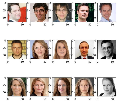
The top row shows examples of economists, who the model didn’t recognize as such.
The center row depicts examples of what the model “thinks” economists look like, but who are actually students / researchers with a different major.
Finally, the bottom row shows examples of good matches, i.e. people for whom the model had a very high confidence for their actual class.
Again, if you are in one of these pictures and want to get removed, please contact me.
Confusion matrix
To see which profession the model is unsure about, I calculated the confusion matrix.
1 | array([[12.76595745, 5.95744681, 0. , 6.38297872], |
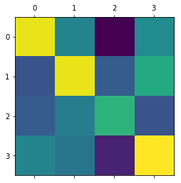
Legend:
- 0 = cs, 1 = econ, 2 = german, 3 = mechanical
- Brighter colors ~ higher value
What we can read from the confusion matrix is that, for instance, the model tends to classify economists as mechanical engineers quite often.
Conclusion
First of all, this is not a scientific study, but rather a small hobby project of mine. Also, it does not have a lot of real-world importance, since one might rarely want to classify students into four categories.
Although the results are not spectacular, I am still quite happy about them and at least my model was able to do a lot better than random guessing. Given an accuracy of 57 % with four classes, you could definitely say that it is, to some extent, possible to learn a stereotypical-looking person’s study major from only in image of their face. Of course, this only holds true within a bounded context and under a set of restrictions, but it is still an interesting insight to me.
Moreover, I am quite sure that there is still a lot of room for improvements to the model, which could yield a better performance. Those might include:
- More training data from a wider range of sources
- More thorough preprocessing (e.g. filter out images of secretaries)
- Different model architecture
- Hyper-parameter tuning
- Manual feature engineering
- …
Please let me know what you think of this project. I would love to get some feedback!